Walkthrough of Typical Xcessiv Workflow
This guide aims to demonstrate the power and flexibility of Xcessiv by walking you through a typical Xcessiv workflow. We’ll optimize our performance on the breast cancer sample dataset that comes with the scikit-learn library.
Starting Xcessiv
First, make sure your Redis server is up and running. In most cases, Redis will be running at its default port of 6379.
Open up your terminal and move to your working directory. Let’s make a directory called XcessivProjects and move inside it:
mkdir XcessivProjects
cd XcessivProjects
XcessivProjects will contain all projects we create with Xcessiv.
To run Xcessiv in the current directory, we simply run:
xcessiv
This will run the Xcessiv server and a single worker process with the default configuration. You can view the Xcessiv application by pointing your browser at localhost:1994 by default.
To view the full range of configuration variables you can configure using the command line, type:
xcessiv -h
For example, to run the Xcessiv server along with 3 separate worker processes, run:
xcessiv -w 3
A note about worker processes
Xcessiv doesn’t do the heavy processing in its application server. Instead, Xcessiv hands the jobs off to separate RQ worker processes. If you have more than one worker process running, then you will be able to process jobs in parallel without any additional configuration. However, keep in mind that each worker will consume its own CPU and memory. The optimal number of workers will then depend on your dataset size, number of cores, and available system memory.
Creating/Opening a Project
When you open Xcessiv for the first time, you’ll see a plain screen and a single button. Click on the button to open the Create New Project modal. This modal provides all functionality needed to create and open an Xcessiv project.

Since XcessivProjects is an empty folder, we won’t see any existing projects yet. Create a new project then open it.
Now would be a good time to explain the structure of an Xcessiv project. An Xcessiv project is essentially a folder with a SQLite database and a sub-folder for storing saved meta-features. When you want to share your project with other people, all you need to do is give them a copy of this folder and they will be able to open it using their own Xcessiv installation. Keep in mind that this folder might get very big for large projects with a large number of saved meta-features.
Importing your dataset into Xcessiv
After opening your new project, the first thing to do is to define your dataset.
Define the main dataset
First, we must define the main dataset.
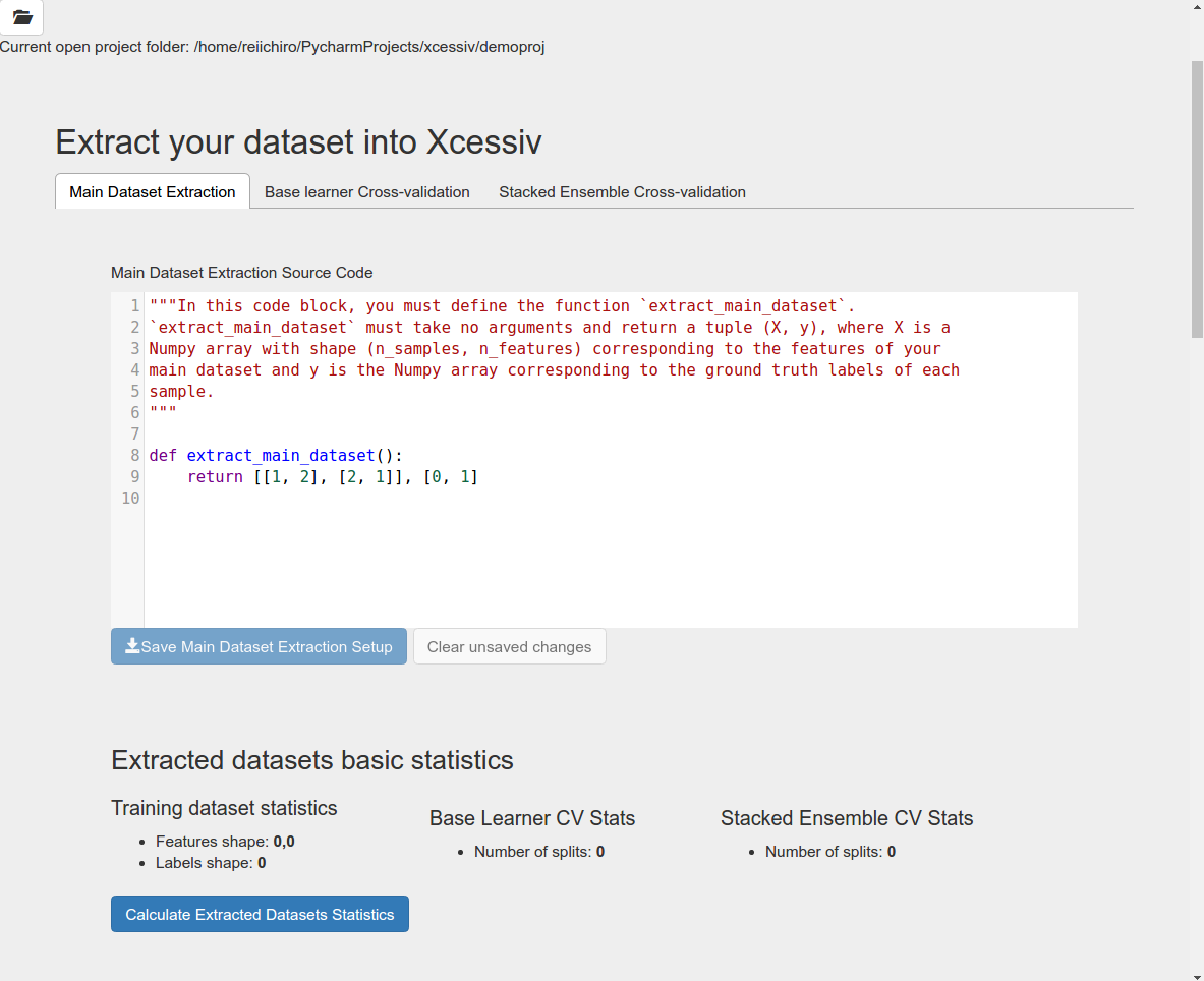
In the code block shown, you must define a function extract_main_dataset() that takes no arguments and returns a tuple (X, y), where X is a Numpy array with shape (n_samples, n_features) corresponding to the features of your main dataset and y is the Numpy array corresponding to the ground truth labels of each sample.
Experienced scikit-learn users will recognize this format as the one accepted by scikit-learn estimators. As a project heavily influenced by the wonderful scikit-learn API, this is a theme that will come up repeatedly when using Xcessiv.
Since we’re going with the breast cancer sample dataset that comes with scikit-learn, copy the following code into the Main Dataset Extraction code block.:
from sklearn.datasets import load_breast_cancer

def extract_main_dataset():
    X, y = load_breast_cancer(return_X_y=True)
    return X, y
Xcessiv gives you the flexibility to extract your dataset any way you want with whatever packages are included in your Python installation. You can open up the quintessential csv file with pandas. Or directly download the data from Amazon S3 with boto. As long as extract_main_dataset() returns the proper format of your data, any way convenient for you will do. One important thing to keep in mind here is that for every process that needs your data, Xcessiv will call extract_main_dataset(). Keeping this function as light as possible is recommended.
Save your dataset extraction code and click the Calculate Extracted Datasets Statistics button. This will look for the extract_main_dataset() function in your provided code block and display the shape of X and y. This is a good way to confirm if your code works properly.
Confirm that X (Features array) has a shape of (569, 30) and y (Labels array) has a shape of (569,).
Define the base learner cross-validation method
After defining the main dataset, we must define how Xcessiv does cross-validation for its base learners. In Xcessiv, the base learner cross-validation’s purpose is two-fold.
First, the cross-validation method is used to calculate the model-hyperparameter combination’s relevant evaluation metrics on the data. Experienced users will recognize this as the usual purpose of cross-validation in machine learning.
Second, the cross-validation method is used to generate the meta-features. Meta-features are the term used for new features generated by the base learners that are used by the second-level learner in stacked ensembling. In most cases, this can be the actual predictions or the output probabilities of each class.
For stacked ensembles, there are two main ways to extract meta-features: cross-validation to get out-of-fold predictions for every sample in the dataset, or having a single train-test split to generate the meta-features (blending). The difference between the two can be found at the Kaggle ensembling guide
For now, all you need to know is that using full cross-validation will allow you to use your whole training set for training the secondary learner at the expense of added computational complexity while using a single train-test split will only train the secondary learner on the meta-features generated from that test split.
Therefore, for smaller datasets, cross-validation is preferred while for larger datasets where computational cost is a real factor, you should use a single train-test split.
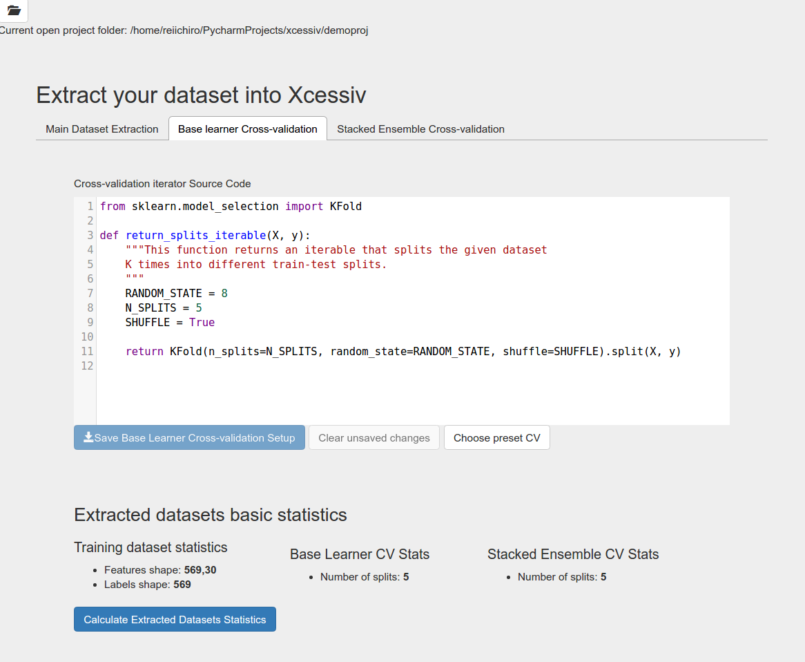
Since the breast cancer dataset has only 569 samples, we will use cross-validation. In the code block shown, copy the following code.:
from sklearn.model_selection import StratifiedKFold

def return_splits_iterable(X, y):
    """This function returns an iterable that splits the given dataset
    K times into different stratified train-test splits.
    """
    RANDOM_STATE = 8
    N_SPLITS = 5
    SHUFFLE = True

    return StratifiedKFold(n_splits=N_SPLITS, random_state=RANDOM_STATE, shuffle=SHUFFLE).split(X, y)
Xcessiv gives you the flexibility to generate cross-validation folds however method you want to. To define a cross-validation method, you must define a function return_splits_iterable() that takes two arguments X and y. These arguments will be passed the X and y variables returned from the previously defined extract_main_dataset() function. return_splits_iterable() will then return an iterator that yields a pair of indices for each train-test split it generates. Again, this is a concept taken straight out of the scikit-learn API and as such, most built-in cross-validation iterators from scikit-learn will work. See http://scikit-learn.org/stable/modules/cross_validation.html#cross-validation-iterators for the details.
A note about random seeds
It is extremely important that the folds generated by return_splits_iterable() are deterministic. Otherwise, ensembling will not work correctly. Therefore, for any cross-validation iterator that depends on a random state, make sure to set it in the function as well.
The given code does stratified K-Fold validation with 5 train-test splits and a random seed set at 8.
So far, we have given code for defining cross-validation. What if we wanted to do a simple train-test split for generating meta-features (blending)? In that case, it is interesting to note that a single train-test split can be defined by a cross-validation iterator that yields only one pair of indices for a train-test split. You can use either sklearn.model_selection.ShuffleSplit or sklearn.model_selection.StratifiedShuffleSplit with n_splits set to 1 for this functionality. Or, roll your own implementation.
If you click again on Calculate Extracted Datasets Statistics, you will notice that the base learner cross-validation statistics will show you the number of splits generated.
Since most problems will rely on very common cross-validation methods, Xcessiv provides several preset return_splits_iterable() implementations based on existing scikit-learn cross-validation iterators.
Define the stacked ensemble cross-validation method
Since the secondary learner of a stacked ensemble is trained on a different set of features (the meta-features), it is natural to define a separate cross-validation method for it. Under the Stacked Ensemble Cross-validation tab, we see a field extremely similar to the one we found in the previous step.
In fact, to define your cross-validation method for the secondary learner, you also need to define a function return_splits_iterable() with the exact same function signature as before. Keep in mind though, that the X and y arrays passed to this function will be from the meta-features.
In most use cases and for valid comparison with the base learner metrics, you can just use the exact same cross-validation method you used for the base learners.
Go ahead and copy the exact same code we used previously into this code block.:
from sklearn.model_selection import StratifiedKFold

def return_splits_iterable(X, y):
    """This function returns an iterable that splits the given dataset
    K times into different stratified train-test splits.
    """
    RANDOM_STATE = 8
    N_SPLITS = 5
    SHUFFLE = True

    return StratifiedKFold(n_splits=N_SPLITS, random_state=RANDOM_STATE, shuffle=SHUFFLE).split(X, y)
Click on Calculate Extracted Dataset Statistics and you should see that the stacked ensemble cross-validation statistics shows the number of splits at 5.
Defining your base learners and metrics
When you’re satisfied with your dataset extraction and base learner cross-validation setup, the next step is to define your base learners and the metrics by which you will judge the performance of each base learner.
In Xcessiv, a base learner is an instance of a class with the methods fit, get_params, and set_params.
Again, scikit-learn users will recognize that these are methods common across all scikit-learn estimators. In Xcessiv, all scikit-learn estimators can be used straight out of the box with no extra configuration. This is a good thing as well even if you wish to use algorithms from external libraries such as XGBoost or Keras, as these libraries often have scikit-learn compatible wrappers around their core estimators e.g. XGBoostClassifier, KerasClassifier.
Use a basic scikit-learn estimator
Let’s begin by defining a classic scikit–learn estimator, the sklearn.ensemble.RandomForestClassifier.
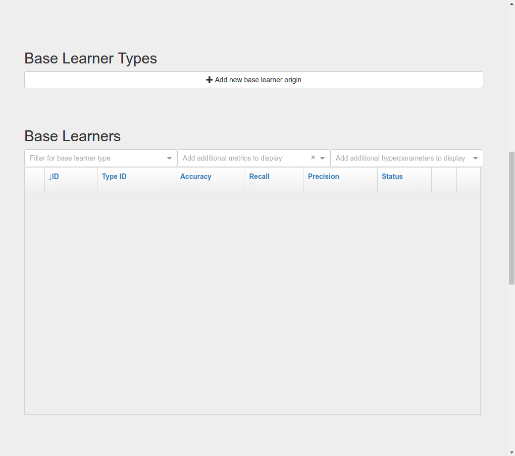
Click the Add new base learner origin button to define a new base learner.
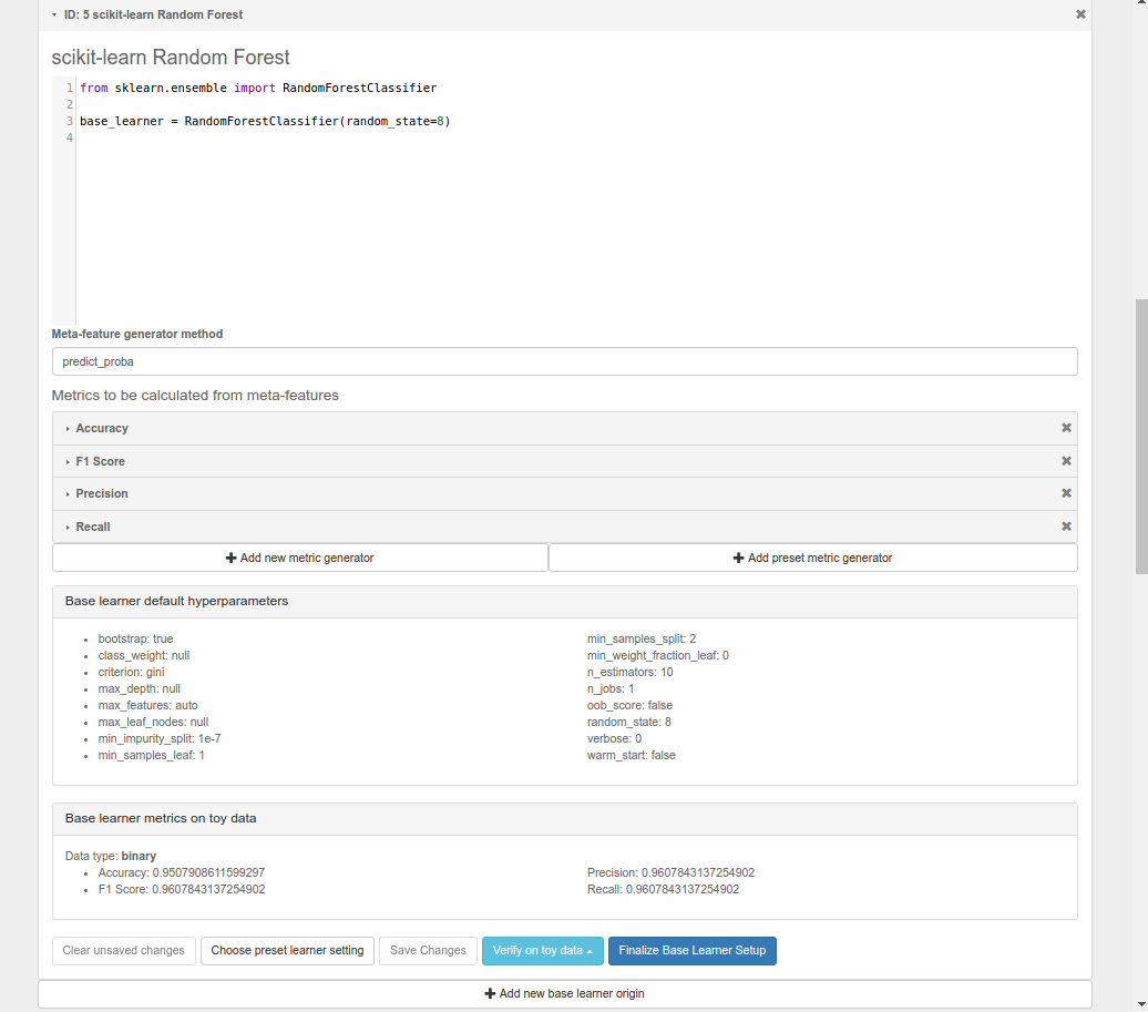
Rename the default name Base Learner Setup to Scikit-learn Random Forest. Then, copy the following code into the code block then save.:
from sklearn.ensemble import RandomForestClassifier

base_learner = RandomForestClassifier(random_state=8)
All it takes to define the base learner is to assign an instance of your estimator class to the variable base_learner.
You will notice that we initialized the Random Forest’s random_state parameter with a value of 8. We want base_learner initialized with the default parameters we want it to have.
Why random_state? Since we will be storing the performance of our base learners, we want any estimators with a randomized element to run the same way every time. Estimators with the same hyperparameters except for the random seed should still be considered different estimators. It is good practice to set any random seeds in base_learner with a deterministic value
Use the scikit-learn pipeline object for more advanced estimators
An incredibly useful tool for chaining together different transformers and estimators is the scikit-learn sklearn.pipeline.Pipeline object. If you want an in-depth guide to pipelines, see http://scikit-learn.org/stable/modules/pipeline.html.
Create another base learner origin, rename it to PCA + Random Forest, and copy the following code into the code block then save.:
from sklearn.pipeline import Pipeline
from sklearn.ensemble import RandomForestClassifier
from sklearn.decomposition import PCA

estimators = [('pca', PCA(random_state=8)), ('rf', RandomForestClassifier(random_state=8))]
base_learner = Pipeline(estimators)
Here we’ve defined a pipeline of PCA followed by Random Forest and assigned it to base_learner. This is now considered a single base learner type whose hyperparameters are a combination of PCA hyperparameters and Random Forest hyperparameters.
Again, notice how we’ve initialized all random seeds to a fixed value.
Predefined base learners
Xcessiv contains predefined base learners for the some of the more common base learners such as Random Forest and Logistic Regression.
You can click the Choose preset learner setting button to view and use predefined base learners.
Define the meta-feature generator method for a base learner
Up to now we’ve defined estimators that have fit methods for training on a train data set, and get_params and set_params for getting and setting hyperparameters, respectively.
But we haven’t yet defined what method base learners use to generate the meta-features. For classifiers, the most common way to generate meta-features is either predict or predict_proba. By default, Xcessiv sets the meta-feature generator method to predict_proba.
For estimators that don’t have the predict_proba method, you can change the meta-feature generator to whatever you want. For example, for SVM classifiers, it is recommended to use decision_function instead of predict_proba because of the additional computational complexity in when probabilities are generated.
Whatever you choose to be the meta-feature generator method, it must take a single variable X, where X is an array-like object of shape (n_samples, n_features), and return a Numpy array of shape (n_samples,) or (n_samples, num_meta_features), where num_meta_features is a positive integer referring to the number of meta-features generated per sample e.g. 5 for predict_proba in a dataset with 5 unique classes. In other words, the estimator must take every sample and decompose it into a single meta-feature e.g. predict, or a set of meta-features e.g. predict_proba.
This flexibility allows you to do things like using regressors as base learners for classifier ensembles, or even PCA-transformed features as meta-features.
Define your metrics
To quantify the “goodness” of a base learner, we’ll need to define metrics to evaluate the quality of its generated meta-features.
For classifiers, very common metrics include Accuracy, Recall, and Precision. For regression, a useful metric is Mean Squared Error.
Other important metrics include the Area Under Curve of the Receiver Operating Characteristic (AUC-ROC) or the Brier Score, both of which can be calculated through the class probabilities output of a classifier.
Let’s define an Accuracy metric for our Random Forest base learner.
Click the Add new metric generator button. Name it Accuracy. In the resulting code block, add in the following code and save:
from sklearn.metrics import accuracy_score
import numpy as np

def metric_generator(y_true, y_probas):
    """This function computes the accuracy given the true labels array (y_true)
    and the scores/probabilities array (y_probas) with shape (num_samples, num_classes).
    For the function to work correctly, the columns of the probabilities array must
    correspond to a sorted set of the unique values present in y_true.
    """
    classes_ = np.unique(y_true)
    if len(classes_) != y_probas.shape[1]:
        raise ValueError('The shape of y_probas does not correspond to the number of unique values in y_true')
    argmax = np.argmax(y_probas, axis=1)
    y_preds = classes_[argmax]
    return accuracy_score(y_true, y_preds)
To define a metric, you must define a function metric_generator that takes two arguments. The first argument should take an array-like object referring to the set of true labels, in this case, y_true, with shape (num_samples,). The second argument should take an array-like object with shape (num_samples, num_meta_features) corresponding to the generated meta-features per sample, y_probas. The value returned should be the calculated value of the particular metric.
The function above calculates the Accuracy metric from the ground truth labels and the corresponding set of class probabilities returned by a classifier.
In the case that our meta-feature generator method is set to predict, this would be the correct code for calculating Accuracy:
from sklearn.metrics import accuracy_score

metric_generator = accuracy_score
Like predefined base learners, Xcessiv comes with a bunch of preset metric generators for some commonly-used metrics. You can use and reuse these for the most common use cases instead of writing your own function every time you define a base learner.
You can add as many valid metrics as you want. These will be calculated every time the base learner is processed. Let’s go ahead and add preset metric generators “Recall from Scores/Probabilities”, “Precision from Scores/Probabilities”, and “F1 Score from Scores/Probabilities” with the Add preset metric generator button.
Save your changes.
Verify your base learner definitions and metrics
After defining your base learners and evaluation metrics, we’ll want to ensure they work as expected.
Xcessiv provides verification functionality that takes your base learner and calculates its metrics on a small sample dataset.
You can choose from toy datasets such as MNIST (multiclass classification), the Wisconsin breast cancer dataset (binary classification), Boston housing prices (regression), and many more. Xcessiv also gives you an option to verify your learner against a custom dataset. You should select a sample dataset with properties that most closely resembles your actual dataset.
Since for this example, we’ll be using our estimator on the breast cancer dataset, we’ll want to verify it on, well, the breast cancer dataset. Click the Verify on toy data button and select Breast cancer data (Binary). If nothing went wrong with your setup, you’ll be able to see your base learner’s hyperparameters with their default values, and the base learner’s metrics on the sample data.
When doing an actual project, you’ll want to verify your base learner on a sample dataset with the closest possible characteristics to your actual data.
Finalize your base learner
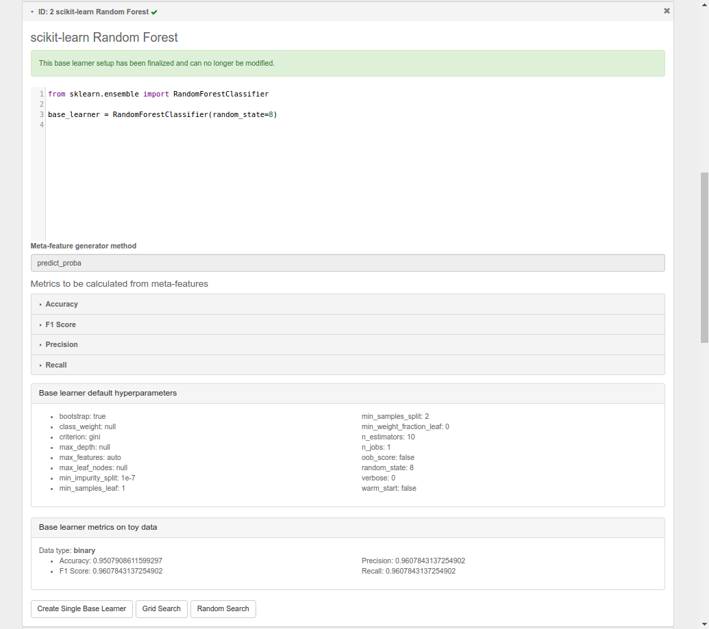
Once you’re happy with your base learner and metrics, there is one last step before you can start testing it on actual data: finalization.
Finalizing locks your base learner setup, after which you will no longer be allowed to make any changes to it. This ensures consistency during the generation of meta-features and metrics while optimizing hyperparameters and creating stacked ensembles.
After finalization, your base learner setup should look like this.
At this point, feel free to create and play around with different learners and metrics. Make sure to verify and finalize all your base learners so you can use them in the next step. For the rest of this guide, I’ll assume you’ve created and finalized a Logistic Regression base learner and an Extra Trees Classifier base learner. Both are available as preset learners.
Optimizing your base learners’ hyperparameters
Once you’ve finalized a base learner, three new buttons appear in the base learner setup window: Create Single Base Learner, Grid Search, and Random Search.
These buttons let you generate meta-features and metrics for your data while giving you different ways to set or search through the space of hyperparameters.
Again, scikit-learn forms the basis for these search methods. Experienced users should have no problem figuring out how they work. For more details on grid search and random search, see http://scikit-learn.org/stable/modules/grid_search.html.
Single base learner
Let’s begin with evaluating a single base learner on the the data. Open up our Random Forest classifier, and click on the Create Single Base Learner button.
In the code block shown, enter the following code.:
params = {'n_estimators': 10}
For creating a single base learner, the code block only has to define a single variable params containing a Python dictionary. The dictionary should contain the base learner hyperparameters and corresponding values as key-value pairs. Any hyperparameter not included in the dictionary will be left at the default value. In fact, if you pass an empty dictionary to params, a base learner with the default hyperparameters will be run on the dataset.
After clicking Create single base learner, you should immediately be able to see your newly generated base learner in the “Base Learners” list. After about 5 seconds, the spinner should disappear and get replaced with a check symbol, signifying that the processing has finished.
Xcessiv does the following after creation and during processing of the base learner.
- Xcessiv creates a new job and stores it in the Redis queue.
- An available RQ worker reads the job and starts processing.
- The worker loads both the dataset and base learner, and sets the base learner with the desired hyperparameters using
set_params. - The worker generates meta-features using the method defined during dataset extraction (cross-validation or through a separate holdout set).
- Using the newly generated meta-features and ground truth labels, the worker calculates the provided metrics for the given base learner.
- The worker updates the database directly with the newly calculated metrics.
- The worker saves a copy of the meta-features to the Xcessiv project folder. These are used during the ensembling phase.
- The browser polls the Xcessiv server from time to time to see if the job has finished and updates the user interface accordingly.
One significant advantage provided by this architecture is that you don’t need to keep the browser open to see the results later on. As long as the worker itself is not stopped while processing, the corresponding database entry will be updated upon success, and you will be able to view the result when you reopen the Xcessiv web application later.
Grid Search
Doing a grid search is a common way of quickly exploring hyperparameter spaces.
Let’s open up our Logistic Regression classifier.
Click Grid Search, and enter the following code.:
param_grid = [{'C': [0.01, 0.1, 1, 10, 100]}]
Five new base learners should be created, with C values of 0.01, 0.1, 1, 10, and 100 respectively.
The format of param_grid should be exactly as that described in http://scikit-learn.org/stable/modules/grid_search.html#exhaustive-grid-search.
Now, reopen the Grid Search modal and re-enter the parameter grid you ran previously. You’ll see that your request is successful but no new base learners are actually created. Xcessiv automatically detects whether a previous model-hyperparameter combination has already been processed and skips it. You don’t need to worry about overlapping grid search spaces.
Remember that this is Python code, so if you’re feeling creative, you can also enter things like:
param_grid = [{'C': range(10)}]
Random Search
Randomized parameter optimization is also a popular method of searching hyperparameters.
On our Extra Trees Classifier, click Random Search, and enter the following:
from scipy.stats import randint
from scipy.stats import expon

import numpy as np

np.random.seed(8)

param_distributions = {'max_depth': randint(10, 100),
                       'min_weight_fraction_leaf': expon(scale=.1)}
Enter 4 in the Number of base learners to create field.
Four new base learners should be created, with random values for max_depth and min_weight_fraction_leaf, sampled from the given scipy distributions.
param_distributions should be a dictionary whose format is described in detail in http://scikit-learn.org/stable/modules/grid_search.html#randomized-parameter-optimization.
By default, the scipy distributions will return different values every time you run the random search because it is, well, random. However, if you set the Numpy global random seed using np.random.seed(), you’ll be able to exactly reproduce random searches.
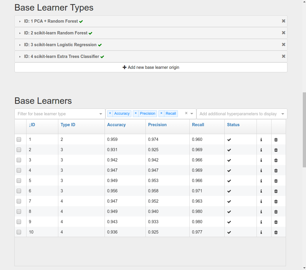
At this point your list of base learners should look like this.
Bayesian Search
As of v0.3.0, Xcessiv includes an experimental automated hyperparameter tuning functionality based on Bayesian search. For the purposes of this initial walkthrough, we will skip this and move on to the next section. A detailed tutorial for using Bayesian optimization can be found in Bayesian Hyperparameter Search.
Creating a stacked ensemble
If you followed all steps up to now, you’d have 10 base learners. In practice, you’d probably try a lot more than ten but for now, let’s go ahead and stack them together using a second-level classifier.
You can add base learners to your ensemble through their checkbox, or by manually selecting their IDs.
Let’s select the highest performing base learner from each base learner type. For stacked ensembles, it’s good to have as much variance as possible in your meta-features. One way to ensure that is to use as many different types of base learners as you can.
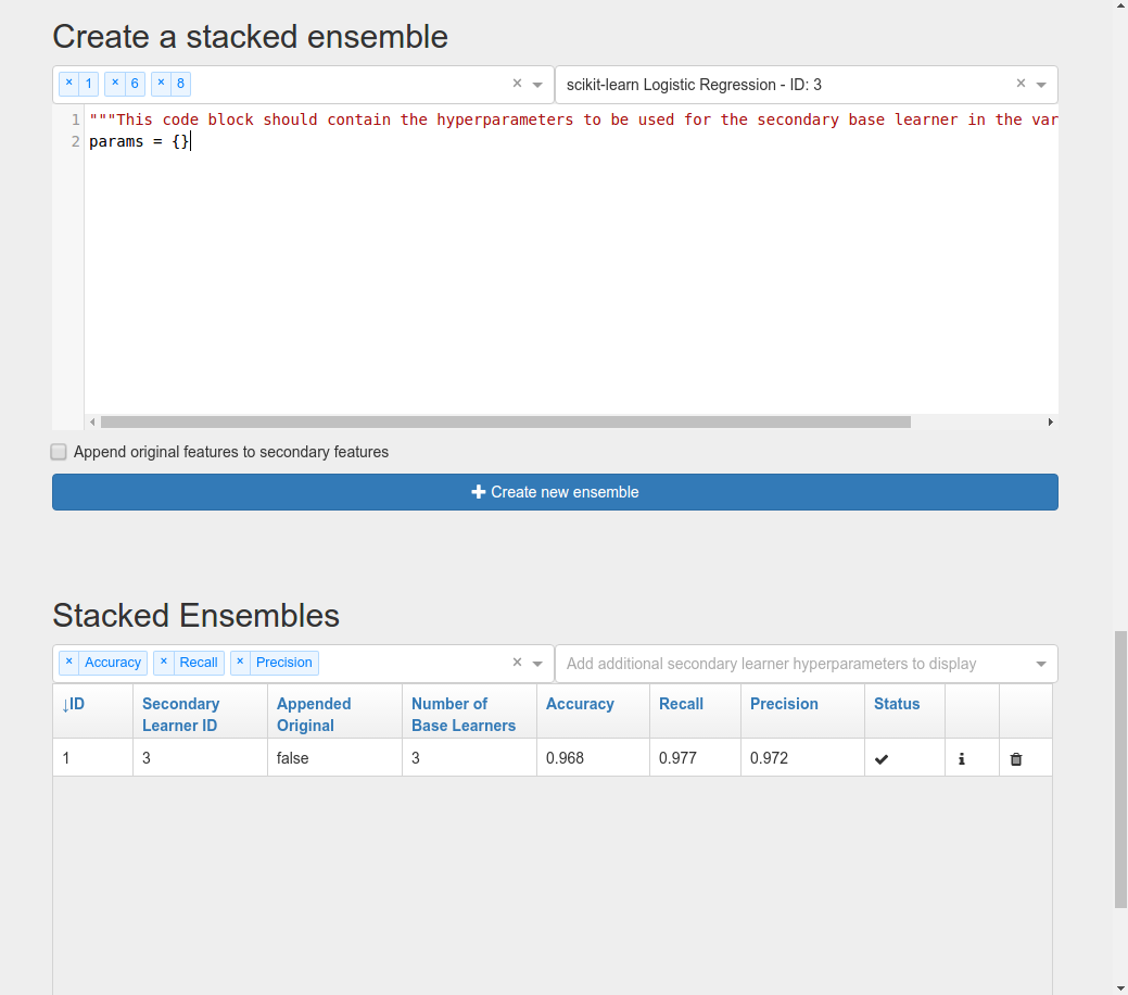
In the Select secondary base learner to use dropdown list, choose Logistic Regression as your secondary classifier. You can use anything you want here of course, but let’s keep things simple for now.
To set the hyperparameters of the secondary learner, enter the following into the code block.:
params = {}
This should keep the Logistic Regression at its default values. If you’ll notice, the format required for this code block is exactly the same as that required when creating a single base learner.
After a short time, your ensemble should finish processing, and you’ll be able to see its performance. Here we get an accuracy of 0.968, which is higher than any individual base learner.
Here’s a complete list of what happens when Xcessiv creates a new ensemble. Note that it is very similar to what Xcessiv does when processing a base learner.
- Xcessiv creates a new job and stores it in the Redis queue.
- An available RQ worker reads the job and starts processing.
- The worker loads the secondary learner class and selected base learners’ saved meta-features from the project folder, and sets the secondary learner with the desired hyperparameters using
set_params. - The worker concatenates the meta-features, and if selected, the original features, together to create the new feature set.
- Using the cross-validation method you set for Stacked Ensemble Cross-validation, the secondary base learner’s metrics on the new feature set are calculated.
- The worker updates the database directly with the newly calculated metrics.
- The browser polls the Xcessiv server from time to time to see if the job has finished and updates the user interface accordingly.
And that’s it! Try experimenting with more base learners, appending the original features to the meta-features, and even changing the type of your secondary learner. Push that accuracy up as high as you possibly can!
Normally, it would take a lot of extraneous code just to set things up and keep track of everything you try, but Xcessiv takes care of all the dirty work so you can focus solely on the important thing, constructing your ultimate ensemble.
Exporting your stacked ensemble
As a Python file
Let’s say that after trying out different stacked ensemble combinations, you think you’ve found the one. It wouldn’t be very useful if you didn’t have a way to use it on other data to generate predictions. Xcessiv offers a way to convert any stacked ensemble into an importable Python file. Click on the export icon of your chosen ensemble, and enter a unique name to save your file as.
In this walkthrough, we’ll save our ensemble as “myensemble.py”.
On successful export, Xcessiv will automatically save your Python file inside your project folder.
Your ensemble can then be imported from myensemble.py like this.:
# Make sure myensemble.py is importable
from myensemble import base_learner
base_learner will then contain a stacked ensemble instance with the methods get_params, set_params, fit, and the ensemble’s secondary learner’s meta-feature generator method. For example, if your secondary learner’s meta-feature generator method is predict, you’ll be able to call base_learner.predict() after fitting.
Here’s an example of how you’d normally use an imported ensemble.:
from myensemble import base_learner

# Fit all base learners and secondary learner on training data
base_learner.fit(X_train, y_train)

# Generate some predictions on test/unseen data
predictions = base_learner.predict(X_test)
Most common use cases for base_learner will involve using a method other than the configured meta-feature generator. Take the case of using sklearn.linear_model.LogisticRegression as our secondary learner. sklearn.linear_model.LogisticRegression has both methods predict() and predict_proba(), but if our meta-feature generator is set to predict(), Xcessiv doesn’t know predict_proba() actually exists and only base_learner.predict() will be a valid method. For these cases, base_learner exposes a method _process_using_meta_feature_generator() you can use in the following way.:
from myensemble import base_learner

# Fit all base learners and secondary learner on training data
base_learner.fit(X_train, y_train)

# Generate some prediction probabilities on test/unseen data
probas = base_learner._process_using_meta_feature_generator(X_test, 'predict_proba')
As a standalone base learner setup
You’ll notice that base_learner follows the scikit-learn interface for estimators. That means you’ll be able to use it as its own standalone base learner. If you’re crazy enough, you can even try stacking together already stacked ensembles.
In fact, Xcessiv has built in functionality to directly export your stacked ensemble as a standalone base learner setup.
In the Export ensemble modal, simply click on Export as separate base learner setup. A new base learner setup will be created containing source code for the selected stacked ensemble. At this point, you’ll be able to use it just like any other base learner. Rename it, add any relevant metrics, tune it, and stack it!
Warning
Xcessiv’s export functionality works by simply concatenating the source code for the different base learners and your cross-validation scheme. While this is not a problem in most cases, things can break. For example, if a base learner’s source code starts with from __future__ import, it will not end up on the first line and this will need to be manually edited out in the exported file.